Terrestrial gravimetry surveys have been carried out for many years, aiding in the search for oil and other natural resources. These have typically been large area surveys (the order of kilometres) looking for large gravity signals (milliGals; 10^-5 ms^-2). Now, with the promise of step change sensitivity from portable atom interferometer (AI) gravity gradiometers, we can think of surveying the gravity gradient on much smaller scales, seeking vastly smaller targets.
Inference (or more commonly ‘inversion’) from gravity data is known to suffer from the problem of ambiguity, meaning that there are many possible (theoretically infinitely many) underground models for a given gravity data-set obtained above ground. As a result of this, we wish to limit the model space to models which are compatible with any a-priori information that we might have. Bayes’ theorem provides a natural means to achieve this through the prior distribution.
We can update our a-priori information with information contained within the gravity data, to obtain posterior inference of model parameters. However, with this approach for high dimensional models (i.e. large number of model parameters) the computation of the posterior distribution becomes mathematically intractable. As a result the posterior must be estimated using stochastic algorithms such as Markov chain Monte Carlo (McMC).
An example of Bayesian inference from one line of gravity data (solid red line) taken above a nuclear bunker is shown in Figure 1.
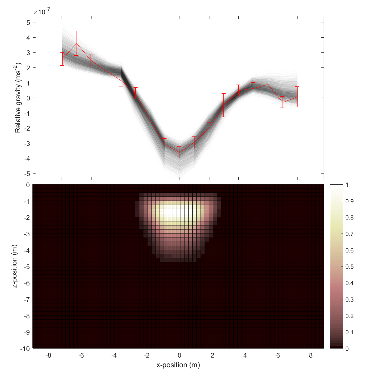 Figure 1: Accepted models from the McMC algorithm are plotted in transparent black. The spatial extent of the anomaly is shown by the colour map, where lighter squares represent higher posterior probability of the anomaly being located at that point. The red square shows the true anomaly position.