An introduction to the statistical modelling of climate change: 1850-2020

by Marco G. Ercolani 

This article is a beginner’s guide to modelling climate change by statistical methods. We will see how data spanning 1850-2020 can be used to model global warming.[1]

In the first part of this article, we comment on graphs of climate data. These data include global temperatures, atmospheric carbon dioxide, solar activity and particulates in the stratosphere. These variables have been chosen because they are of interest to both climate change doubters and believers.

In the second part of this article, we fit statistical models to these data to estimate the amount by which each variable has affected global temperatures during 1850-2020. The models indicate that increased atmospheric carbon dioxide can explain 1.26 to 1.33 degrees Celsius of the temperature increase while cyclical solar activity can explain about 0.12 to 0.40 degrees of the temperature increase.

The third part of this article includes instructions on how to estimate two statistical models of climate change using an Excel spreadsheet.

A final section summarises and is followed by data and a technical appendix.

It is worth noting that statistical models (see http://www.climateeconometrics.org) are rarely used in climate modelling. Instead, experimental and physical models are more often used, such as the simulations run by meteorologists. In these models, the parameters are decided upon by the researcher based on various sources, such as laboratory experiments, meteorological readings or the results of statistical models. These physical models are then used to run simulations to verify whether the simulations closely match the observed world. In contrast, statistical models are fitted directly to the observable data to determine their parameters. Both approaches are equally valid and both produce mathematical models that can be used to forecast climate change. 

The data

In this first section, we look at graphs of the climate data as a preliminary step before estimating the statistical models in section two. The Data Sources Appendix includes details of the data sources.

Figure 1 shows an overall temperature increase of about 1.5 degrees Celsius since 1850. The period 1850-1940 seems one of gradual temperature increase. The Second World War was a period of relatively high temperatures but followed by a period between 1945-1964 when temperatures did not increase substantially. The period since 1965 has been one of rapid temperature increase. There are smaller year-on-year fluctuations but it is difficult to determine which of these are real fluctuations and which are measurement errors. Smoothing the year-on-year fluctuations is a bad idea because it would erase some important variations. For example, 1877 and 1878 have remarkably high temperatures during a major El Niño episode in what was dubbed ‘the year without a Winter’. Conversely, there are some years with sudden temperature dips and these coincide with major volcanic ejecta into the stratosphere.

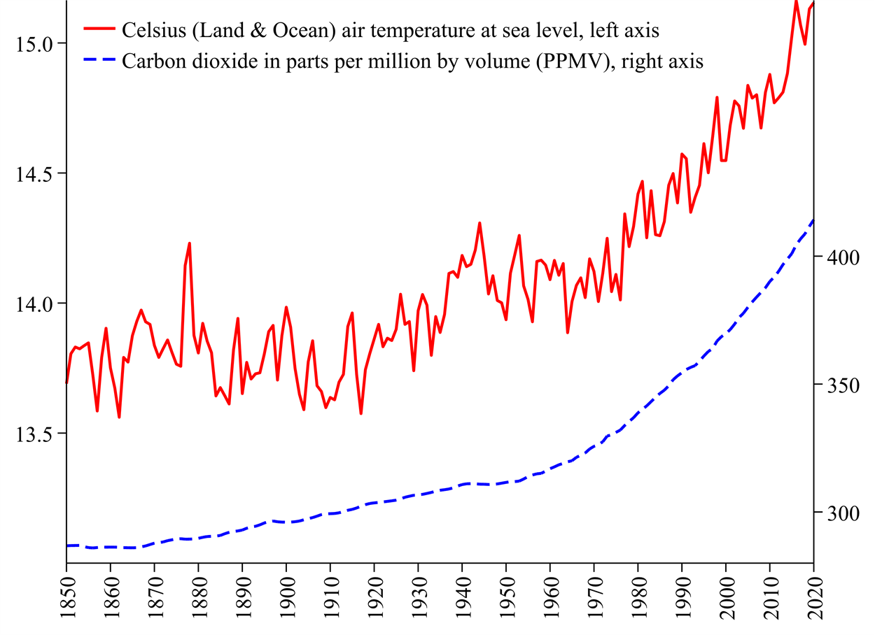
Figure 1: Average global annual temperatures and atmospheric carbon dioxide, 1850-2020

Figure 1 also illustrates the levels of atmospheric carbon dioxide, a major greenhouse gas.[2] Greenhouse gasses work by allowing high-frequency sunlight energy into the troposphere but blocking much of the lower-frequency heat energy from escaping. The scientific consent is that increased temperatures are mainly due to increased greenhouse gasses. Atmospheric carbon dioxide has increased by just over a third since 1850.

Figure 2 illustrates sunlight energy reaching Earth, measured as Total Solar Irradiance (TSI) in kilowatts per square metre (kW/m²). TSI has a short cycle of about 11 years that coincides with planetary alignments.  Solar TSI is included in our models but this is unlikely to explain much of the temperature increase because the overall fluctuation in TSI is a relatively small 0.18% with just a 0.0025 kilowatt increase relative to a level of about 1.36 kilowatts. We have overlaid a ‘smoothed TSI’ variable on the original one that suggests a two-century cycle but this is hard to confirm with less than two centuries of data. We have also illustrated the ‘Solar (TSI) cycle’ which is the difference between TSI and ‘smoothed TSI’.

Figure 3 illustrates data on solar dimming caused by particulates high in the stratosphere. This is known as Stratospheric Aerosol Optical Dimming (SAOD). SAOD data are measured at the 550nm (nanometre) electromagnetic wavelength. Greater dimming leads to cooling by reducing the sunlight reaching Earth’s surface. These dimming data have several peaks that coincide with major volcanic eruptions. Eruptions with a Volcanic Explosivity Index of 6 have been illustrated[3]  (see  https://en.wikipedia.org/wiki/Volcanic_Explosivity_Index for a definition of the VEI.)

 

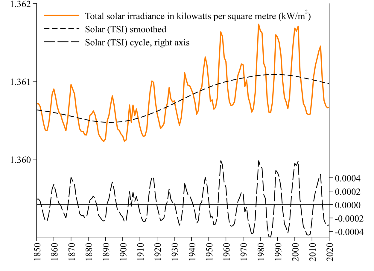
Figure 2: Total Solar Irradiation (TSI) reaching Earth in kilowatts per square metre

 

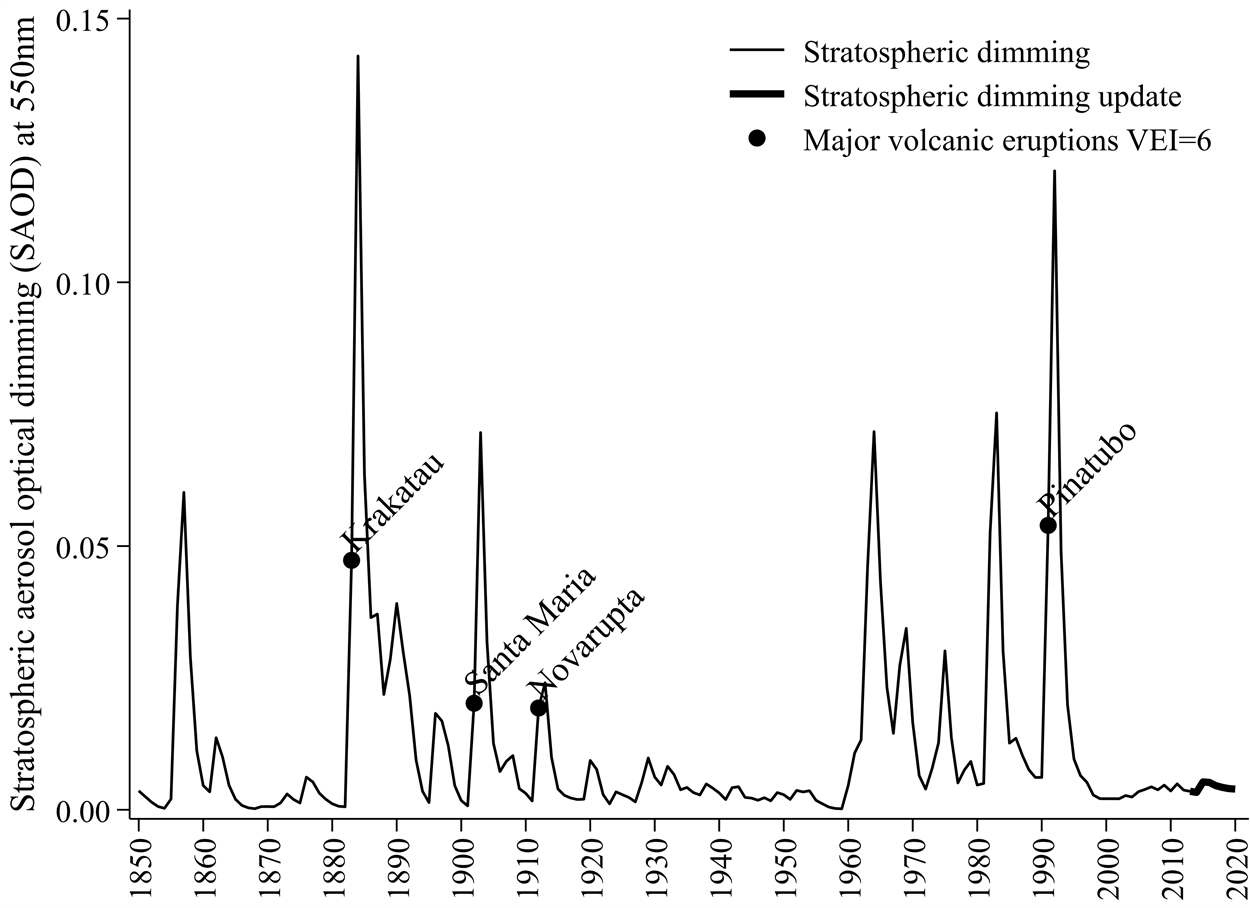
Figure 3: Total Solar Irradiation (TSI) reaching Earth in kilowatts per square metre

The statistical model

In this section we will look at the results of fitting two statistical models to the data using the method of least squares[4]. In particular we use ordinary least squares (OLS), which is the simplest of these methods. OLS involves selecting the model parameters that generate the smallest (squared[5]) difference between the observed temperatures and temperatures fitted by the model. At the end of this section, we will see how to carry out these model estimates using the Excel software.

The first statistical model we fit to our data is on temperatures, carbon dioxide, total solar irradiance (TSI) and stratospheric dimming. The resulting model is:

  Celsius = 0.0104 Carbon dioxide + 48.63 Solar (TSI)

                                                    – 1.79 Dimming + 0.42 El Niño 1877-1878 – 55.4 + e                              (1)

where we have also included a variable for the major El Niño event, set equal to one on 1877 and 1878, and zero elsewhere.

The parameter numbers in model (1) indicate how much each unit of each variable contributed to temperatures. For example, each part per million of carbon dioxide contributes an estimated 0.0104 increase in Celsius temperatures. Since 1850, carbon dioxide has increased by 128.3 parts per million, contributing to an estimated 1.33 (= 0.0104 x 128.3) degrees to the temperature increase. Solar irradiation also makes a positive contribution of 48.63 degrees per kilowatt. Increased Solar irradiance therefore contributed approximately 0.12 (= 48.63 x 0.0025) of a degree to increased temperatures. The upward dimming spikes illustrated in Figure 3 correspond with temperature falls based on the parameter –1.79. The El Niño 1877-1878 event has a large positive effect on temperatures raising them by 0.42 of a degree over this two-year period. The final parameter –55.4 is a constant that captures all that is missing in the model, such as the temperature effects of atmospheric water vapour or atmospheric methane, ozone and nitrous oxide. In a near-complete model we would have expected this constant term to be close to -273.15, which is absolute zero. Given no model is perfect, the residual errors e in model (1) represent differences between the observed and model-fitted temperatures.

Figure 4 illustrates the temperatures already seen in Figure 1, overlaid with the temperature values fitted from model (1). We can see how good the overall fit in this model is. Figure 4 also reports the squares of the residual errors e in model (1) that were minimised to fit the model. These represent the smallest squared residual errors that could be achieved when fitting the model using the method of ordinary least squares.

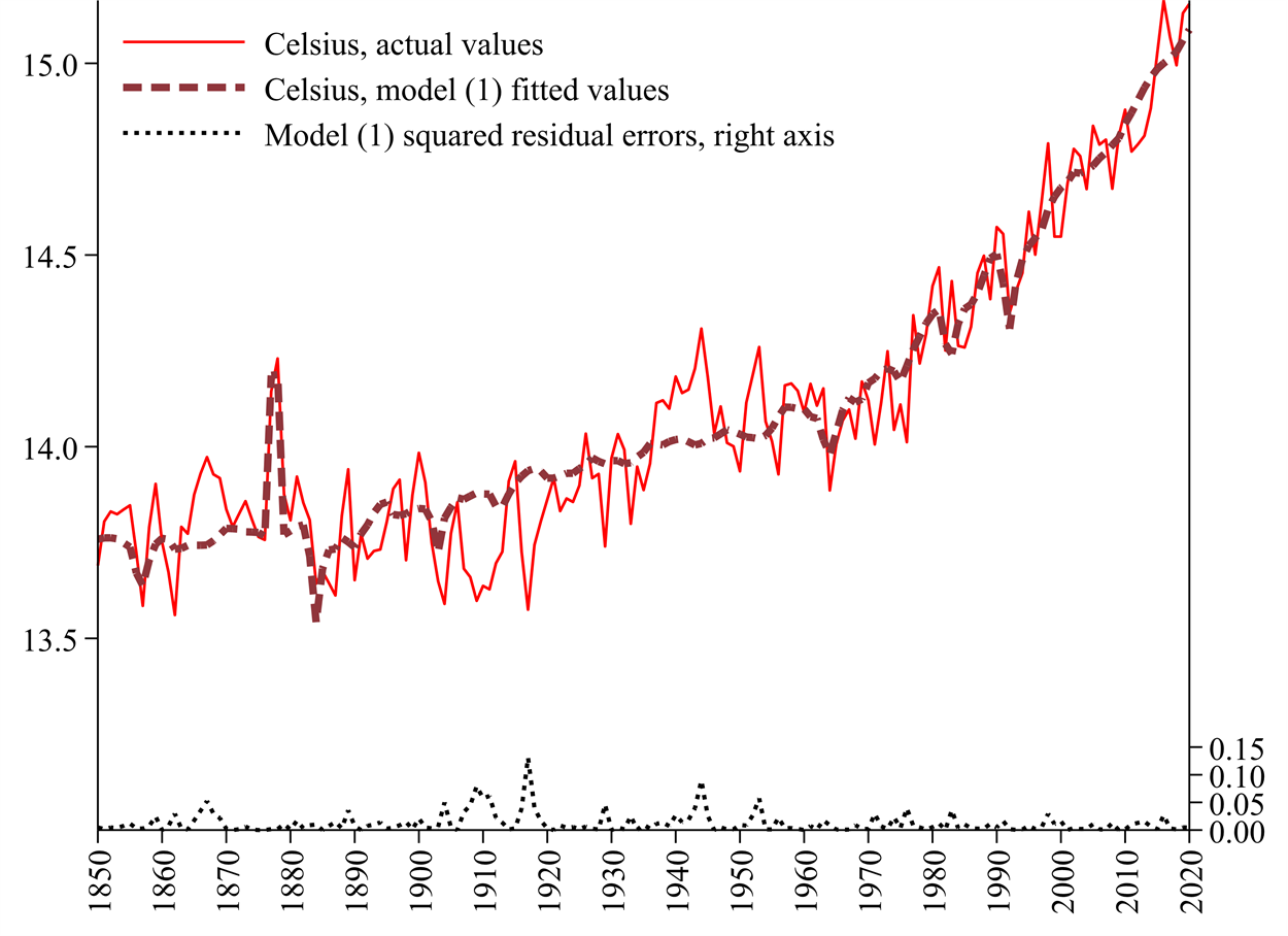
Figure 4: Actual and model (1) fitted Celsius temperatures, and squared residual errors

 

In our second model we split the Solar (TSI) into its smoothed component and its cyclical component already illustrated in Figure 2. The resulting OLS model is:

  Celsius = 0.0098 Carbon dioxide + 161.2 Solar Smooth + 11.31 Solar Cycle
                                              – 1.87 Dimming +0.425 El Niño 1877-1878 – 208.4 + e                                (2)

Model (2) is very similar to model (1) with carbon dioxide explaining an estimated 1.26 (= 0.0098 x 128.3) degrees of the temperature increase. The main difference is the separate parameters on the two solar activity variables. The parameter on ‘Solar Smooth’ is 161.2, suggesting a stronger influence than in model (1). Model (2) suggests increased Solar irradiance has contributed approximately 0.40 (=161.2 x 0.0025) of a degree to increased temperatures. The parameter on the 11-year Solar Cycle is much smaller at 11.31, suggesting a very small effect. 

How to fit a statistical model using Excel

Models such as (1) and (2) can be estimated using any statistical software (such as R, SPSS or Stata) and can even be carried out using spreadsheet programs such as Excel.  Your estimated results are likely to differ very slightly from those in this article because the data are being continually fine-tuned and your dataset might not span the same years.

Most people will probably have access to Excel and wish to use it to estimate their models. First make sure that the Excel ‘statistical add-ins’ are activated by selecting: File, Options, Add-ins, Go; and then make sure the ‘Analysis ToolPak’ and ‘Analysis ToolPak (VBA)’ options are ticked. To estimate equation (1) select: Data, Data Analysis, Regression[6] and OK to launch the ‘Regression’ box illustrated in Figure 5. In the “Input Y Range” box insert the column with Celsius. In the “Input X range” box, insert the columns for Carbon dioxide, Dimming and Solar. If you included the variable labels when selecting the data ranges, tick the box for “Labels”. Then click OK and this should place a new estimated model into a new worksheet in the same Excel workbook. You can repeat a similar process to estimate model (2) but might need to reposition some data columns to achieve this.

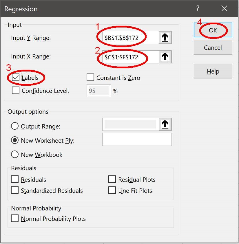
Figure 5: Excel ‘Regression’ box used to estimate statistical models. 

Summary

This article has shown us how to estimate a statistical model of climate change. In the first section we have seen various climate variables and gained an initial insight into how they might be interrelated. In the second section we have seen how to use Ordinary Least Squares model-fitting to estimate two models of climate change. All of the proposed climate variables have some impact on the temperature increase experienced since 1850 but by far the greatest contribution comes from increased atmospheric carbon dioxide. The article appendices touch on data sources some advanced topics when it comes to statistical models of time-series data. 

Data Sources Appendix

Temperature data in Figure 1 are from Berkeley Earth (http://BerkeleyEarth.org) Land and Ocean temperatures at sea level, developed by Rohde and Hausfather (2020, https://doi.org/10.5194/essd-12-3469-2020). Berkley Earth describes itself as “Independent, non-governmental, and open-source” and was originally established to look into the “merit[s] in some of the concerns of climate skeptics”.

Post 1959 carbon dioxide data in Figure 1 are based on atmospheric air readings at the Mauna Loa Observatory in Hawaii, made available by the Global Monitoring Laboratory (https://www.esrl.noaa.gov/gmd/). Historical carbon dioxide data are based on numerous polar deep ice-core readings (https://www.ncdc.noaa.gov/data-access/paleoclimatology-data/datasets/ice-core) by MacFarling Meure et al. (2006, https://doi.org/10.1029/2006GL026152).

In Figure 2, recent TSI data spanning 1978-2020 by Coddington et al. (2015, https://doi.org/10.7289/V55B00C1) are based on satellite readings and were retrieved from www.ncdc.noaa.gov/cdr/atmospheric/total-solar-irradiance. Two historical TSI datasets by Marvel et al. (2015, https://doi.org/10.1038/nclimate2888) and Miller et al. (2014, https://doi.org/10.1002/2013MS000266) were retrieved from https://data.giss.nasa.gov/modelforce/solar.irradiance. Where the TSI data overlap, we use an average of the readings.

Figure 3 solar dimming data spanning 1850-2012, with updates to Sato et al. (1993, https://doi.org/10.1029/93JD02553), were retrieved from http://data.giss.nasa.gov/modelforce/strataer/ using the last available dataset tau.line_2012.12.txt. These are constructed from volcanic ejecta, terrestrial readings and satellite readings. We constructed the missing 2013-2020 data by using detailed monthly data on volcanic eruptions retrieved from the Smithsonian Institution Global Volcanism Program using their data retrieval tool: https://volcano.si.edu/search_eruption.cfm and supplemented with data by Siebert et al. (2010, Volcanoes of the World) from www.allcountries.org/ranks/volcano_explocivity_index_ranks.html.

 

Advanced Statistical Appendix

In this appendix we touch on some important but advanced issues related to statistical model estimation. The first issue is related to ensuring the estimated models are not spurious regressions and the second issue is to construct valid significance test statistics on the estimated parameters.

The first issue is that it is easy to fit statistical models to data that are non-stationary, such as ever-increasing temperatures. To demonstrate that the statistical model is not a spurious regression we need to demonstrate that its residual errors are mean-reverting. This is typically done using unit root tests of non-stationarity. Applying the most commonly used one of these, the “Augmented” Dickey and Fuller (1981, https://doi.org/10.2307/1912517) (ADF) test to the residual errors of models (1) and (2) produces the following test statistics. These indicate the two models are super-consistent, cointegrated and not spurious because the residual errors are mean-reverting:

ADF test on model (1) residual errors, t-statistic = -7.4455, p-value = 0.000007

ADF test on model (2) residual errors, t-statistic = -7.5684, p-value = 0.000024

The p-values, based on MacKinnon (2010, https://www.econ.queensu.ca/research/working-papers/1227), indicate strong rejection of non-stationarity of the error-residuals.

The second issue is that we typically wish to test whether each model parameter is equal to zero and this is based on standard t-statistics. However standard t-statistics are not valid because some of the variables are non-stationary. Various corrections are possible and we apply the Engle and Yoo (1987, https://doi.org/10.1016/0304-4076(87)90085-6) three-stage estimation correction. The first stage includes the models already reported in models (1) and (2) but the t-statistics are not valid. The second stage (not reported) includes error-correction models with three-year lags of first-differenced temperatures and carbon dioxide among the regressors. The third stage involves adjusting the first stage results based on second-stage correction results. The first-stage (i) and third stage (iii) results for models (1) and (2) are reported in Table 1.

	Dependent variable: Celsius temperatures
	in Engle-Yoo (1987) models
	Model 1						Model 2
	(1.i)			(1.iii)			(2.i)			(2.iii)
Regressors:	Param.	t-stat		Param.	t-stat		Param.	t-stat		Param.	t-stat
Carbon dioxide	0.0104	35.77***		0.0107	15.95***		0.0098	24.43***		0.0093	10.46***
Dimming	-1.790	-4.16***		-4.78	-4.87***		-1.872	-4.38***		-4.831	-5.16***
El Nino1877-1878	0.420	5.20***		0.970	5.29***		0.425	5.32***		0.956	-5.04***
Solar (TSI)	48.63	1.75		69.30	1.10
Solar Smooth							161.2	2.76**		329.7	2.59**
Solar Cycle							11.31	0.35		-18.32	-0.26
Constant	-55.40	-1.47		-65.97	-2.05**		-208.4	-2.63**		-298.4	-4.38***
R2	91.5%						91.7%

Probability of having erroneously included this parameter ^* p < 0.05, ^** p < 0.01, ^*** p < 0.001.

Table 1: Engle and Yoo (1987) first stage (i) and third stage (iii) model (1) and (2) estimates

The Table 1 results confirm that most of the variables are statistically significant in explaining global Celsius temperatures. Only the Solar activity variable is not significant in models (1.i) and (1.iii) but this might be because the short 11-year cycles are masking the effect of the long fluctuation. When Solar activity is split into its smoothed fluctuations and its short Solar Cycles, we see that the smoothed component is significant in explaining temperature changes. In all the models, carbon dioxide remains the most significant variable in explaining global warming.